 |
OGLE Basic Tutorial |
by Michael J. Gourlay
http://www.cora.nwra.com/Ogle/
by Michael J. Gourlay http://www.cora.nwra.com/Ogle/ |
Contents:
The Ogle web site has software and data needed to run Ogle and to go through this tutorial.
In addition to the Ogle source code, the OpenGL, GLUT, MUI, GLUI and zlib libraries are also required. If your system lacks OpenGL, Mesa can replace it, but Ogle requires 3D hardware acceleration to perform satisfactorily.
Visit these web sites for packages used to compile Ogle:
Instructions for compiling and installing Ogle are included with the Ogle source code.
From the Ogle tutorial-files directory, download these files:
With a text editor, look at the "tutorial.ogle" command file. Notice how simple it is. The format of the command file is described in the Ogle manual page, which should be installed online on your machine. The Ogle manual page is also available from the main web site through the "Information" link.
(The data for this tutorial is fictitious, although you could
interpret the data as a vortex in a divergent field.)
Ogle accepts these command line options:
Ogle uses a toolkit called "GLUT", which understands these additional
command line options:
Execute this command:
Two windows will pop up: The Ogle Render Window and the Ogle
Controls.
Starting Ogle
| - | Ogle Render Window | · | |
|---|---|---|---|
 | |||
| Ogle Controls | |
|---|---|
 |
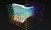
Initially the Ogle Render Window will only contain a bounding box,
three axes, and a status window at the bottom. To view the data, one
or more dataviews must be active and you will activate those later.
The controls for manipulating the view, however, can be used even when
no dataviews are active.
Select the Ogle Render window so that it has focus. Now press any of
the following keys: i, h, j, k, l, m. Pressing these keys will rotate
the object. Pressing ";" will reset the orientation to look along the
minus z-axis with the x-axis to the right and the y-axis upward.
You can also use the mouse to rotate the object by clicking on the
checkered sphere in the Ogle Control Panel and moving the mouse.
Pressing the following keys will translate the object: a, s, d, f, e,
x. Pressing "q" will reset the translation. Notice that the
translation widgets in the Ogle Controls window will change when the
translation keys are used. The translation widgets with arrows in the
Ogle Controls window can also be used to translate the object.
Ogle separates the scale into 4 components: The relative x, y and z
scales, and the "all" scale. The relative scales effectively set the 3D
aspect ratio of the object, and those values always lie in the range of
zero to one. The "all" scale is a factor applied to all three directions
uniformly and changes the size of the object. Press "-" or "=" to alter
the "all" scale for the object.. Pressing "[Backspace]" will reset the
"all" scale. Notice that "scale" widgets in the Ogle Controls will
update when the scale keys are pressed. The scale widgets can also be
used to scale the object. The scale widgets also allow for the object
to be scaled differently in each of the canonical directions, x, y and z.
Holding the "[Shift]" key while using the keyboard controls will make
the increment of change smaller. For example, pressing "H" will rotate
the object less than, but in the same direction as, pressing "h".
During the rest of the tutorial, as various display and data parameters
are changed, try rotating, scaling, and translating the object to see
it from various views.
Click the checkbox labeled "Stereoscopic" to change whether
stereoscopic rendering is on or off. When stereoscopic rendering is
on, red/cyan glasses can be worn to make the display look
three-dimensional. The cyan filter should cover the left eye and the
red filter should cover the right eye. Note that stereoscopic
rendering mode can be toggled from within the application but on some
platforms, stereoscopic rendering will not work correctly unless the
"-stereo" command line option was provided when starting Ogle.
Click the "Orthographic projection" checkbox to toggle between
perspective and orthographic projection. Perspective projection looks
more realistic, but orthographic projection will not distort the size
of the object based on its distance from the viewer.
Click the "Clip plane" checkbox to turn on or off the clip plane. The
clip plane is parallel to the viewing screen, and located at the
origin. The clip plane can be made to intersect the object at any
plane by translating the object along the viewing direction (the "z"
direction) and by rotating the object. This is one way to view
cross-sections of data.
Click the "axes", "subset box" and "bounding box" checkboxes to change
whether the coordinate axes, subset box and data bounding box are
drawn. The "subset box" only appears when a dataview is active, and
later this tutorial will describe dataviews or subsets.
Click the "Write view image" button to write a copy of the current
display to an image file. The image files are named "ogle-xxx.ppm"
where "xxx" is a serial number starting at 000. The image file format
is PbmPlus Portable Pixmap, which is extremely simplistic, and supported
by most image processing software.
In the Ogle Controls window, press and hold "Show Dataview
controls...". A menu of dataviews will pop up. Select "Opacity
Renderer". A window alled "Opacity Renderer Controls" will pop up.
Orientation
Options
Commands
Dataviews
| Opacity Renderer Controls | |
|---|---|
 |
In the "Opacity Renderer Controls" window, press the checkbox labeled "Active". Now press the "Apply" button. The render window will display a volume rendering of the data.
Press the "Active" checkbox to deactive the opacity renderer. Press "Apply" to update the display. The volume rendering will disappear from the Ogle Render Window. Now activate the volume renderer again and update the render window display.
Press the "Hide" button to make the Opacity Renderer Controls
disappear. Now press "show control panels" in the Ogle Controls to
bring back the "Opacity Renderer Controls" window.
In the Ogle Controls, press and hold the "data files:" button. This
will pop up a listbox of data filenames. The data filename text box
will show the currently selected filename from the command file.
To read a data file, move the mouse to an entry in the listbox and
release the mouse button.
To update the display, press an "Apply" button in any of the dataview
control windows, change the orientation of the object in the Ogle
Render Window, or change a display parameter in the Ogle Controls.
Select the "0064" data set, and update the display. The initial data
file should have been the "0016" data set, so selecting and displaying
the "0064" data set should cause a higher resolution data volume will
appear in the Ogle Render Window.
Note that the data filenames ends in ".gz" (indicating that this file
has been compressed by gzip). Even though the "tutorial.ogle" command
file omits the ".gz" suffix, Ogle detects this automatically and
decompresses the file on the fly.
Aside from saving disk space (in this case by a factor of about 8),
using a compressed data file is also faster than reading the
uncompressed file since uncompressing speed is usually faster than disk
IO speed, especially for disk IO across a network.
Note that the ".ogle" command file can list the filename without the
".gz" suffix whether or not the filename actually has a ".gz" suffix.
If the file has ".gz" then Ogle will automatically recognize that.
Data Files
Data Compression
| Ogle Render Window | |
|---|---|
 |
In each dataview control window is a set of subset widgets. Each of the x, y and z directions has an associated minimum, maximum and stride widget. These values have integer units of "voxels" corresponding to the number of gridpoints in the data volume, in the range zero to Ni-1 where Ni is the number of gridpoints in theith direction. Slowly change some of the subset widgets. Notice that the Ogle Render Window stops displaying the dataview and shows only the bounding boxes and axes (assuming that the "axes", "subset box" and "bounding box" checkboxes are checked). The status window will also indicate that the view is not current. Also notice that there are two bounding boxes: one bright and one dim. The bright subset bounding box changes shape when the subset minimum and maxium widgets are changed. The dim box always shows the full dimensions of the data volume.
The stride indicates the amount by which to decimate the data, in each direction. For some dataviews, changing the stride is useful to speed rendering. In other dataviews, increasing the stride can decrease the amount of graphic objects rendered, making the view simpler and easier to understand.
To update the display with the new subset, press the "apply" button in any dataview control window, change the orientation of the object, or change some display parameter in the Ogle Controls.
Set the 'subset y' and 'subset z' minimum values to be 0 and the
maximum values to be the largest possible. Set the 'subset x' minimum
to be 0 and the 'subset x' maximum to be half of the maximum possible.
Update the display. Half of the data volume will appear, with the other
half sliced off.
In the Opacity Render Control window, press and hold the left-most
colormap "type" listbox (below to the colormap legend). Move the mouse
to the entry labeled "red-cyn-0.color / center-0.alpha" and release the
mouse button. The colormap legend will change. The "red-cyn-0.color /
center-0.alpha" colormap is an external one indicated in the command
file. The other colormaps are built into Ogle. Press "Apply" to
update the display.
Ogle applies gamma correction to colormaps, to correct for nonlinear
responses of displays. Ideally, your display will have its gamma
calibrated but in practice people rarely perform this calibration, so
Ogle performs a rudimentary gamma correction. This is controlled by the
command line option "-gamma g" where "g" is the gamma correction value.
When image files are written, they have the gamma correction applied
to them. If those images are then viewed on a display with a different
gamma correction value then the image will look different.
In the Opacity Render Control window, change the "selected variable" to
be "-1" (which means to use the magnitude of a vector quantity instead
of a particular component). Press the colormap type button until it
indicates "spike", and press "Apply". The spike colormap effectively
selects a narrow band of data values, similar to the effect of an
isosurface, but fuzzier. Change the "spike width" and "spike center"
parameters. The colormap legend will contintually update to show the
current spike size and position. Press the "Apply" button to update
the renderer display.
The values of "selected variable" typically correspond to the components
of the data set, and have values in the range zero to Nv-1
where Nv is the number of data components in the data set.
Change the "opacity multiplier" widget to be 0.2 and update the render
window display. The volume rendering will apear more translucent.
Usually an opacity multiplier value of 1.0 is appropriate. Set the
"opacity multiplier" to 0.5 and update the display again. Later in the
tutorial the translucency effect will demonstrate how volume renderings
interact with other forms of dataviews.
Colormaps
| Vector Field Controls | |
|---|---|
 |
Pop up the "Vector Field Controls" window and make that dataview active. Press "Apply". A number of line segments will appear.
Press the colormap type button until it indicates "hot/cold signed", and press "Apply". Notice the coloring of the vector field glyphs. Change the "selected variable" control to 1, and press "apply". Notice that the vector field glyphs have the same location and orientation, but their color has changed. The "selected variable" controls which vector data component is used to color the vectors.
In the Vector Field Control window, press the glyph button, and press "Apply" for each glyph type. For each glyph type, rotate the object. Some glyphs are slower to render than others. The "lit cones" glyph will probably be the slowest, but it also usually makes the best image.
| Ogle Render Window | |
|---|---|
 |
Change the "threshold min" and "threshold max" values, and press "Apply" for each setting. Note that the number of vector field glyphs rendered changes for each setting. The threshold values are relative to the data value range for the data component with the largest absolute value. If a vector value at a gridpoint within the data volume has a scaled magnitude between the threshold min and max values, then a glyph is rendered for that gridpoint.
Change the "length scale" value and press "apply" for each setting. Note that the size of the glyphs change. The length scale is relative to the grid spacing, so if the grid is more sparse, the vector glyphs will be larger. Usually a length scale values around 0.6 to 0.7 will yield the best looking images.
Change the "stride" values for the vector field and update the display. Notice that when all stride values are higher, fewer vector glyphs are drawn, and they are proportionally longer. Increasing the stride in a vector field can make the display less cluttered and easier to visualize.
Notice that the vector glyphs on the far side of the volume rendering
are still visible, but partially obscured, as though behind a thin
cloud. This is an interesting feature of volume renderings; they
provide depth cues.
Pop up the "Streamline Controls" window.
Streamlines
| Streamline Controls | |
|---|---|
 |
In the Streamline Control window, change the "subset z" controls so that the min and max are both near the middle value. Change the "subset x" min (but not max) value to be near the middle. Make the streamline dataview active. Change the "subset y" min and max value to be near the middle. Notice that the subset bounding box is updated in the Ogle Render window as it is changed. The subset bounding box for the Streamlines dataview should now be a narrow strip along the x axis.
Press the "apply" button. Several streamlines will be rendered.
Change the Streamline colormap to "spectrum unsigned". Set the "selected variable" to 2. Update the display. The streamlines will be colored according to vector component 2, the z-component.
It will be useful to deactivate all other dataviews to see some of the aspects of streamlines demonstrated in this section of the tutorial.
Change the "length max" control to have a value around 1.0. Change the colormap type to be "magenta/green signed". Press "apply". Colored sections of streamlines will appear in the render window.
Press the direction button until it indicates "forward" and press "apply". The sections of streamline will be rendered in only the forward direction relative to the starting region. Now press the direction button until it indicates "backward" and press "apply". The sections of circle will be rendered in the opposite direction relative to the starting region. The direction can also be "bidirectional".
Change the "length max" to a value around 3. The "length max" controls the maximum length of each direction of a streamline. Values are scaled by the domain size, so a value of 1.0 will yield streamlines no longer than the length of the longest dimension of the box. Note that if the streamline curves quite a bit that a length of 1.0 probably will not extend the length of the box. In fact, streamlines that reconnect to themselves will never occupy more than some finite length regardless of the "lemgth max" setting.
Change the line width and line pattern, pressing apply after each setting. Notice that the streamlines are rendered differently for each such selection.
The "decimation" value controls how many points along the streamlines are rendered. If the decimation is 1 then all points along the streamline are rendered. If the decimation is 10 then every 10th point is rendered. Increasing the decimation will increase the rendering speed but decrease the apparent smoothness of the rendered lines. The decimation does not change the streamline integration routine, but only the rendering. Set the decimation to 100 and press "apply". Notice that the streamlines appear chunky. Set the decimation to 1 or 2 and press "apply" to render more smooth streamlines.
The "step min", "step max" and "error tolerance" controls determine the behavior of the integration routine which generates the streamline. Usually there will be no reason to change the default values. If the streamlines take too much time to generate, then increase the "step min" or "error tolerance" values. Beware that this also diminishes the accuracy of the streamlines.
Notice that the DataView controls contain two streamlines. The reason for this is that you might want to apply different criteria for streamlines, and produce two sets of streamlines. For example, you might want to shoot streamlines through a plane of data, using "local min" for one set and "local max" for the other set of streamlines. You could even use two different colormaps for the two sets of streamlines. You could also apply streamlines to two different vector fields if, e.g., your data volume has 6 components.
Reactivate the Opacity Renderer and Vector Field dataviews to see a combined view of all of the dataviews.
| Ogle Render Window | |
|---|---|
 |
| Isosurface Controls | |
|---|---|
 |
Ogle also provides an isosurface dataview. By now you should be able to infer how to make use of that dataview, but some features deserve mention.
An isosurface is a surface where the data has some spatially constant value. Such a surface would share some qualities with an opacity rendering with a narrow spike colormap.
The "selected variable" indicates the index of the data component variable to use for finding the isosurface. As usual, a value of -1 means to use the magnitude of a vector quantity.
The colormap data component index indicates the index of the data component to use to color the isosurface. This allows the isosurface to show two variables at once. For example the isosurface could be drawn at the location of constant magnitude, but colored with one component of the vector quantity. A value of -1 indicates to use the same data component as indicated by the "selected variable" in which case the entire isosurface would have the same color.
The Isosurface dataview allows for multiple isosurfaces to be drawn simultaneously. For most situations the isosurfaces would probably be nested, making all but one of the isosurfaces occluded by the outermost. When used with a subset, clip-plane, or in any situation where the isosurfaces are not closed surfaces, however, having multiple isosurfaces could be useful for showing multiple contours. The Isosurface Controls provide widgets for specifying multiple isovalues and the number of isosurfaces. All isovalues beyond the number specified with "number of isosurfaces" are ignored.
The "depth of subdivisions" parameter is peculiar to the algorithm used for generating the isosurface geometry. The algorith used is called "dividing cubes" and operates by drawing a single point at each location within the data volume where the algorithm finds the given isovalue. In most situations this would produce a collection of unconnected dots, unless the data volume were extremely dense or the render window extremely small. To fill in the gaps, the algorithm recursively interpolates and subdivides any cubes containing the specified isovalues. The "depth of subdivision" determines the number of recurses. For each subsequent value of that depth, the algorithm subdivides to create 8 times as many cubes in regions which contain the isovalue. A depth of 0 yields no subdivisions. A depth of 1 effectively visits 8 times as many points. A depth of 2 effectively visits 64 times as many points. Subdivision costs CPU time so increment the depth slowly, rendering the volume each value until the isosurface contains no gaps.
The "point size" parameter changes the size of the point drawn. This should be used along with the "depth of subdivisions" to fill in the isosurface. While increasing the depth slows the rendering process exponentially, increasing point size does not. Increasing point size, however, also makes the isosurface chunkier. The user must decide between speed or smoothness.
 |
Try following the Visible Human
example.